Using Named Range in Microsoft Excel
About Named Ranges
Microsoft Excel lets you define a reference for a selection of cells that be used in the future. These references are called Named Range and can be reused in formulas you create in Microsoft Excel. Named Range may be used as an alternative to absolute references.
In this article, we’ll show you how to create Named Range in Microsoft Excel and reuse them on your formulas. To follow along the steps, you may download the file at this link, https://bit.ly/3doKEF1
The Yearly Sales Spreadsheet
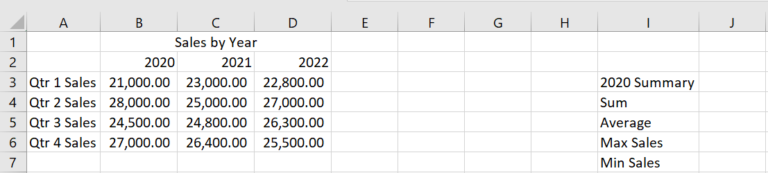
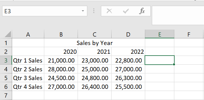
The spreadsheet we’ll be working with contains a breakdown of the quarterly sales for each year 2020-2022. We’ll be getting the summaries for the year 2021. But instead of dragging the same selection of cells or entering an absolute reference for each formula, we’ll create a Named Range for those cells.
Creating the Named Range
The cell address on the formula bar is where we will define the named range for the 2020 sales data. This in turn will be used on the summary formulas.

The first step is to drag the mouse around the cells for the named range, i.e., the 2020 sales data.
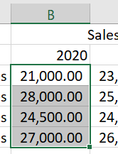
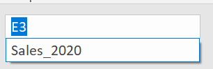
On the cell address, type the text “Sales_2020” and press Enter key on the keyboard- this will now refer to the selected cells i.e., the Named Range.

We’ll do a simple test to see if the Named Range, “Sales_2020” will refer on the selected cells we defined the range on. Click the mouse anywhere on the spreadsheet. The cell address will show where you clicked on.
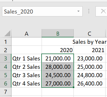
On the cell address, click the drop-down – this will list all the Named Range you have defined.
Click the Named Range, “Sales_2020”. The cells under the range will now be selected.
Using the Named Range in Formulas
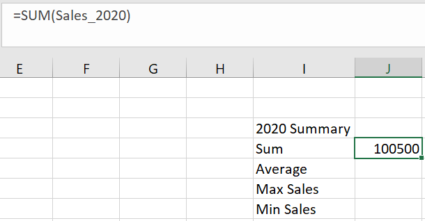
We’ll now use the Named Range for the summary formulas. First, we’ll get the sum of the 2020 sales. Click where the sum will compute. Start by typing the formula “=SUM(“. Right after the open parenthesis, type the first letters for the Named Range. Microsoft Excel will list down “Sales_2020” on its auto complete suggestion. Click the Named Range to select it. Complete the formula with the closing parenthesis and press the Enter key.

The sum for the 2020 sales is computed.
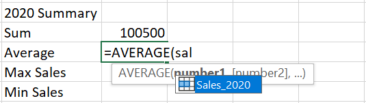
We’ll use the same Named Range to get the average for 2020 sales data. Click where the average will compute. Type the formula “=AVERAGE(“, followed by the first letters for the Named Range. Select “Sales_2020” on the auto complete suggestion. Complete the formula with the closing parenthesis and press the Enter key.
Reusing the Named Range
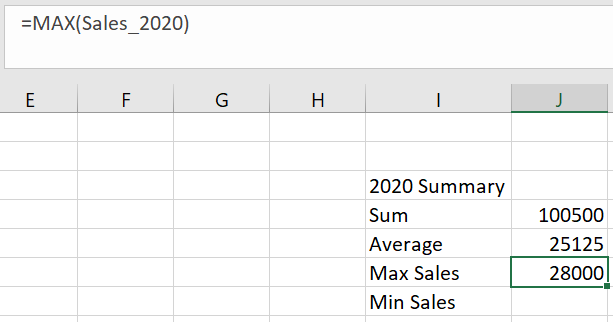
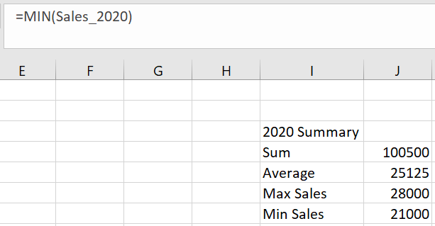
To get the maximum and minimum 2020 sales, the same Named Range can be used to their respective formulas.